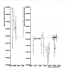
History of measurements of the speed of light; from Henrion and Fischloff, “Assessing uncertainty in physical constants,” American Journal of Physics, September 1986
Reproducibility in modern science
Reproducibility has emerged as a major issue in numerous fields of scientific research, ranging from psychology, sociology, economics and finance to biomedicine, scientific computing and physics. Many of these difficulties arise from experimenter bias (also known as “selection bias”): consciously or unconsciously excluding, ignoring or adjusting certain data that do not seem to be in agreement with one’s preconceived hypothesis; or devising statistical tests post-hoc, namely AFTER data has already been collected and partially analyzed. By some estimates, at least 75% of published scientific papers in some fields contain flaws of this sort that could potentially compromise the conclusions.
Many fields are now undertaking aggressive steps to address such problems. As just one example of many that could be listed, the American pharmaceutical-medical device firm Johnson and Johnson has agreed to make detailed clinical data available to outside researchers, covering past and planned trials, in an attempt to avoid the temptation to only publish results of tests with favorable outcomes.
For further background details, see John Ioannidis’ 2014 article, Sonia Van Gilder Cooke’s 2016 article, Robert Matthews’ 2017 article, Clare Wilson’s 2022 article and Benjamin Mueller’s 2024 article, as well as this previous Math Scholar article, which summarizes several case studies.
Experimenter bias in physics
Physics, thought by some to be the epitome of objective physical science, has not been immune to experimenter bias. One classic example is the history of measurements of the speed of light. The chart on the right shows numerous published measurements, dating from the late 1800s through 1983, when experimenters finally agreed to the international standard value 299,792,458 meters/second. (Note: Since 1983, the meter has been defined as the distance traveled by light in vacuum in 1/299,792,458 seconds.)
As can be seen in the chart, during the period 1870-1900, the prevailing value of the speed of light was roughly 299,900,000 m/s. But beginning with a measurement made in 1910 through roughly 1950, the prevailing value centered on 299,775,000 m/s. Finally, beginning in the 1960s, a new series of very carefully controlled experiments settled on the current value, 299,792,458 m/s. It is important to note that the currently accepted value was several standard deviations below the prevailing 1870-1900 value, and was also several standard deviations above the prevailing 1910-1950 value.
Why? Evidently investigators, faced with divergent values, tended to reject or ignore values that did not comport with the then-prevailing consensus figure. Or, as Luke Caldwell explains, “[R]esearchers were probably unconsciously steering their data to fit better with previous values, even though those turned out to be inaccurate. It wasn’t until experimenters had a much better grasp on the true size of their errors that the various measurements converged on what we now think is the correct value.”
Avoiding experimenter bias in a physics experiment
In a February 2024 Scientific American article, Luke Caldwell described his team’s work to measure the electron’s electric dipole moment (EDM), in an attempt to better understand why we are made of matter and not antimatter. He described in some detail the special precautions that his team took to avoid experimenter error, and, especially, to avoid consciously or unconsciously filtering the data to reach some preconceived conclusion. It is worth quoting this passage at length:
Another source of systematic error is experimenter bias. All scientists are human beings and, despite our best efforts, can be biased in our thoughts and decisions. This fallibility can potentially affect the results of experiments. In the past it has caused researchers to subconsciously try to match the results of previous experiments. … [Caldwell mentions the speed of light controversy above.]
To avoid this issue, many modern precision-measurement experiments take data “blinded.” In our case, after each run of the experiment, we programmed our computer to add a randomly generated number—the “blind”—to our measurements and store it in an encrypted file. Only after we had gathered all our data, finished our statistical analysis and even mostly written the paper did we have the computer subtract the blind to reveal our true result.
The day of the unveiling was a nerve-racking one. After years of hard work, our team gathered to find out the final result together. I had written a computer program to generate a bingo-style card with 64 plausible numbers, only one of which was the true result. The other numbers varied from “consistent with zero” to “a very significant discovery.” Slowly, all the fake answers disappeared from the screen one by one. It’s a bit weird to have years of your professional life condensed into a single number, and I questioned the wisdom of amping up the stress with the bingo card. But I think it became apparent to all of us how important the blinding technique was; it was hard to know whether to be relieved or disappointed by the vanishing of a particularly large result that would have hinted at new, undiscovered particles and fields but also contradicted the results of previous experiments.
Finally, a single value remained on the screen. Our answer was consistent with zero within our calculated uncertainty. The result was also consistent with previous measurements, building confidence in them as a collective, and it improved on the best precision by a factor of two. So far, it seems, we have no evidence that the electron has an EDM.
Caldwell’s data blinding technique is quite remarkable. If some variation of this methodology were adopted in other fields of research, at least some of the problems with experimenter bias could be avoided.
Experimenter bias in finance
The field of finance is deeply afflicted by experimenter bias, because of backtest overfitting, namely the usage of historical market data to develop an investment model, strategy or fund, especially where many strategy variations are tried on the same fixed dataset. Note that this is clearly an instance of the post-hoc probability fallacy, which in turn is a form of experimenter bias (more commonly termed “selection bias” in finance). Backtest overfitting has long plagued the field of finance and is now thought to be the leading reason why investments that look great when designed often disappoint when actually fielded to investors. Models, strategies and funds suffering from this type of statistical overfitting typically target the random patterns present in the limited in-sample test-set on which they are based, and thus often perform erratically when presented with new, truly out-of-sample data.
As an illustration, the authors of this AMS Notices article show that if only five years of daily stock market data are available as a backtest, then no more than 45 variations of a strategy should be tried on this data, or the resulting “optimal” strategy will be overfit, in the specific sense that the strategy’s Sharpe Ratio (a standard measure of financial return) is likely to be 1.0 or greater just by chance, even though the true Sharpe Ratio may be zero or negative.
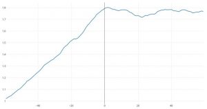
Comparison of index average excess return versus broad U.S. stock market: hypothetical growth of $1 over 60 months before and 60 months after inception of the index.
Data from Joel M. Dickson, Sachin Padmawar and Sarah Hammer, “Joined at the hip: ETF and index development,” July 2012, https://www.vanguardcanada.ca/documents/joined-at-the-hip.pdf.
Some commonly used techniques to compensate for backtest overfitting, if not used correctly, are also suspect. One example is the “hold-out method” — developing a model or investment fund based on a backtest of a certain date range, then checking the result with a different date range. However, those using the hold-out method may iteratively tune the parameters for their model until the score on the hold-out data, say measured by a Sharpe ratio, is impressively high. But these repeated tuning tests, using the same fixed hold-out dataset, are themselves tantamount to backtest overfitting.
One dramatic visual example of backtest overfitting is shown in the graph at the right, which displays the mean excess return (compared to benchmarks) of newly minted exchange-traded index-linked funds, both in the months of design prior to submission to U.S. Securities and Exchange Commission for approval, and in the months after the fund was actually fielded. The “knee” in the graph at 0 shows unmistakably the difference between statistically overfit designs and actual field experience.
For additional details, see How backtest overfitting in finance leads to false discoveries, which is condensed from this freely available SSRN article.
P-hacking
The p-test, which was introduced by the British statistician Ronald Fisher in the 1920s, assesses whether the result of an experiment is more extreme than what would one have given the null hypothesis. However, the p-test, especially when used alone, has significant drawbacks, as Fisher himself warned. To begin with, the typically used level of p = 0.05 is not a particularly compelling result. In any event, it is highly questionable to reject a result if its p-value is 0.051, whereas to accept it as significant if its p-value is 0.049.
The prevalence of the classic p = 0.05 value has led to the egregious practice that Uri Simonsohn of the University of Pennsylvania has termed p-hacking: proposing numerous varied hypotheses until a researcher finds one that meets the 0.05 level. Note that this is a classic multiple testing fallacy of statistics, which in turn is a form of experimenter bias: perform enough tests and one is bound to pass any specific level of statistical significance. Such suspicions are justified given the results of a study by Jelte Wilcherts of the University of Amsterdam, who found that researchers whose results were close to the p = 0.05 level of significance were less willing to share their original data than were others that had stronger significance levels (see also this summary from Psychology Today).
Along this line, it is clear that a sole focus on p-values can muddle scientific thinking, confusing significance with size of the effect. For example, a 2013 study of more than 19,000 married persons found that those who had met their spouses online are less likely to divorce (p < 0.002) and more likely to have higher marital satisfaction (p < 0.001) than those who met in other ways. Impressive? Yes, but the divorce rate for online couples was 5.96%, only slightly down from 7.67% for the larger population, and the marital satisfaction score for these couples was 5.64 out of 7, only slightly better than 5.48 for the larger population (see also this Nature article).
Perhaps a more important consideration is that p-values, even if reckoned properly, can easily mislead. Consider the following example, which is taken from a paper by David Colquhoun: Imagine that we wish to screen persons for potential dementia. Let’s assume that 1% of the population has dementia, and that we have a test for dementia that is 95% accurate (i.e., it is accurate with p = 0.05), in the sense that 95% of persons without the condition will be correctly diagnosed, and assume also that the test is 80% accurate for those who do have the condition. Now if we screen 10,000 persons, 100 presumably will have the condition and 9900 will not. Of the 100 who have the condition, 80% or 80 will be detected and 20 will be missed. Of the 9900 who do not, 95% or 9405 will be cleared, but 5% or 495 will be incorrectly tested positive. So out of the original population of 10,000, 575 will test positive, but 495 of these 575, or 86%, are false positives.
Needless to say, a false positive rate of 86% is disastrously high. Yet this is entirely typical of many instances in scientific research where naive usage of p-values leads to surprisingly misleading results. In light of such problems, the American Statistical Association (ASA) has issued a Statement on statistical significance and p-values. The statement concludes:
Good statistical practice, as an essential component of good scientific practice, emphasizes principles of good study design and conduct, a variety of numerical and graphical summaries of data, understanding of the phenomenon under study, interpretation of results in context, complete reporting and proper logical and quantitative understanding of what data summaries mean. No single index should substitute for scientific reasoning.
Overcoming experimenter bias
Several suggestions for overcoming experimenter bias have been mentioned in the text above, and numerous others are in the linked references above. There is no one silver bullet. What is clear is that researchers from all fields of research need to take experimenter bias and the larger realm of systematic errors more seriously. As Luke Caldwell wrote in the Scientific American article mentioned above:
Gathering the data set was the quick part. The real challenge of a precision experiment is the time spent looking for systematic errors — ways we might convince ourselves we had measured an eEDM when in fact we had not. Precision-measurement scientists take this job very seriously; no one wants to declare they have discovered new particles only to later find out they had only precisely measured a tiny flaw in their apparatus or method. We spent about two years hunting for and understanding such flaws.
[This was originally published at the Math Scholar blog.]