Kelly’s formula is a theoretical benchmark for deciding the appropriate position size when gambling. A divergence in attitude towards this theory illustrates the disconnect between academicians and practitioners, and the necessity of closer collaboration between the two circles, a point we argued in The Two Towers of Finance.
To understand the essence of Kelly’s formula, let us consider the question: Can one lose money in a game in which one has a favorable probability of winning? The answer is, absolutely yes. To see why, think of the simple game of tossing a biased coin: heads means that the player wins the bet, and tail that he loses. Even when the player has a 90% winning probability, if he bets all he has every time, then sooner or later he will inevitably encounter one losing game and go bankrupt. This is a simplified example of gambler’s ruin. Yet, since the odds are so much in favor of the player, it is unreasonable not to play. The reasonable middle ground between not playing and playing is to come up with an optimal bet size. Kelly’s formula determines such an optimal size.
Sketching the log return per play in such a game as a function of the bet size (as a percentage f of the total wealth of the player), we get the picture in the figure below.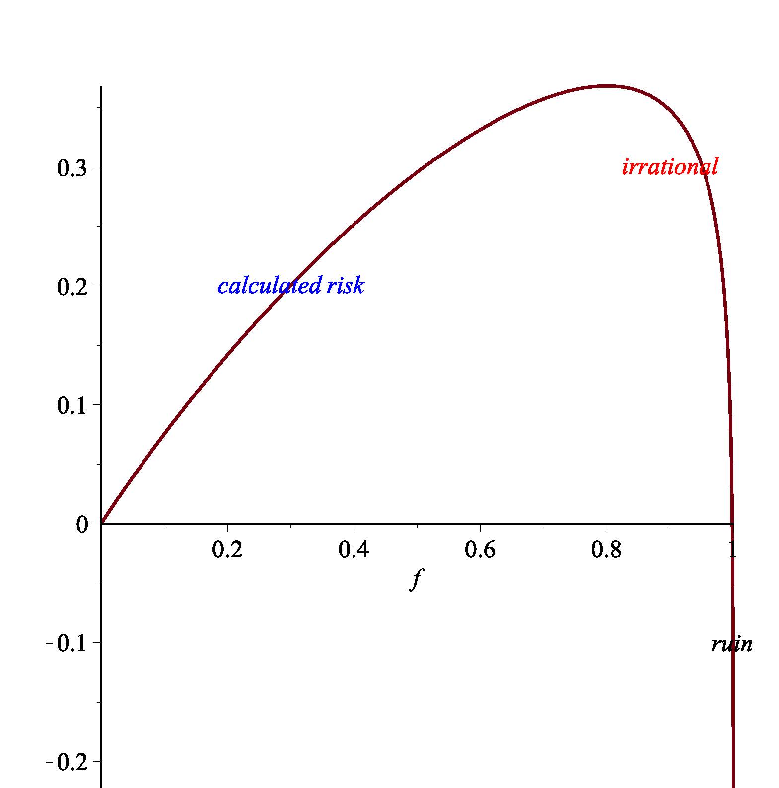
The log return function is essentially what Kelly employed to solve for the unique optimal betting percentage. In our example we can observe the theoretical optimal bet size to be 80%. In general, in such a coin-toss game, if the probability of winning and losing are p and q=1-p, respectively, then Kelly’s formula tells us the theoretical optimal betting size should be p-q, or 2p-1.
More interesting is that Kelly was motivated to explain Shannon’s information rate in information theory. As a result, the average optimal log return at the Kelly’s bet size is actually proportional to the information rate, and can be viewed as the information in this game favorable to the player. The subsequent development of this important result within the circles of practitioners and academicians is rather interesting.
Practitioners regard the Kelly bet size as a red line that should never be crossed. In fact, experienced traders and investors have long known the importance of being conservative in allocating capital into risky assets, even without knowing the Kelly’s formula. They have learned from trial and error — although many seem to have forgotten this principle during the past two decades.
Coming back to our coin toss game, if we used the bet size of 80%, then (with probability 0.1) in one losing game you could loss 80% of your total wealth. If you are unlucky and encounter two losing games consecutively, the total loss will be 96%. Gamblers with a little common sense don’t need any formula to know this is too risky. Thus, for practitioners, Kelly’s formula provides a useful guide for the upper bound of allocating capital to the risky assets. The emphasis has always been how to reduce the risk from there.
Edward Thorp, a mathematics professor turned legendary blackjack player and the pioneer of the basic system for playing blackjack, was a leading practitioner of the Kelly’s formula. He first applied Kelly’s formula in managing bet size in blackjack and later generalized the principle to money management in trading. Thorp’s view is representative of that of a practitioner. Recently, answering a question on whether he uses the Kelly’s formula in asset allocation, he replied, if you bet half the Kelly amount, you get about three-quarters of the return with half the volatility. So it is much more comfortable to trade. I believe that betting half Kelly is psychologically much better.
Indeed, recent research of Vince and Zhu shows that when incorporating the practical consideration of adjusting for risk, and realizing that one only gambles over a finite horizon of time, Kelly’s suggested bet size needs to be adjusted down considerably. This confirms what practitioners have long been doing in the real world.
For many decades, Kelly’s formula was dismissed as irrelevant by leading academics. These included Nobel Prize Laureate Paul Samuelson, who went as far as calling the Kelly criterion a fallacy, and derided it in an article consisting entirely of one-syllable words (presumably so that his benighted opponents could understand it). This led to the bitter Samuelson controversy, which positioned Markowitz’s portfolio theory against the Growth Optimal Portfolio (GOP), each side claiming superiority over the other.
This controversy seems fueled more by partisanship (economists vs. mathematicians) than by practical considerations. Some of the most successful investors have reportedly applied the Kelly criterion, including Warren Buffett and Bill Gross. The caveat is that to construct and to manage the growth portfolio (or alternatively the Markowitz portfolio), one needs to know the joint probability distribution of the price processes of all the assets involved. This is of course a tall order. In practice, all one has to work with is the price history of the assets involved, which is used to estimate the true joint probability distribution. However, searching for optimal strategies through historical simulations leads to the trap of backtest overfitting (see our paper Pseudo-Mathematics and Financial Charlatanism: The Effects of Backtest Overfitting on Out-of-Sample Performance).
These two tales of Kelly’s formula illustrate the dangers of naively following theoretical financial results in investment practice. This is not to say that theoretical results are not useful. For example, the Sharpe ratio, which was developed in the context of Markowitz’s portfolio theory, has become an industry standard in measuring the (past) performance of mutual funds and hedge funds. Similar usage of the idea of the growth portfolio is also useful, especially given the close relationship between the Kelly formula and information theory. As always, caveat emptor!